Learner’s Guide to Dynamic Programming#1
Dynamic programming is an algorithmic problem solving paradigm focused on recognization and elimination of repetitive computation. For this article, I’ll write a short introduction to dynamic programming, and move on to explaining how I try to look at dynamic programming problems.
Introduction to Dynamic Programming
Dynamic programming rests on two simple properties of the algorithms and the problems it works on.
Firstly, a problem needs to have optimal substructure property , namely the property that it is possible to use results of an algorithm for a substructure to compute the results of an algorithm for the whole structure. Let’s demistify this a bit.
Let us look an implementation of array sum algorithm. One would write is as given below in Python in the iterative way.
def sum(array):
  res = 0
  for i in array:
    res += i
  return i
If we instead took the functional way to write it, it could look as below.
def sum(array):
  if array == []:
    return 0
  return array[0] + sum(array[1:])
Even though this looks like a simple change, it’s actually a fundamentally different solution. In the iterative version, if we were to try to put it in natural language, would basically say “Start with 0, add each element to the result, at the end of the array we will have all of them added to the result” while the second one would say “Empty array has a sum of 0, for any non-empty array, we can take the first element and the result of summing the rest, and just add those.
So, if we have a list of items [3, 2, 7, 6], the first algorithm would sum it as
((((0 + 3) + 2) + 7) + 6)
Whereas the second algorithm would sum it as
(3 + (2 + (7 + (6 + 0))))
The real difference between them is, the second one explicitly relies on optimal substructure property . It follows the statement that we can just add the current number with the sum of the rest and the sum of the current array. I believe this line of thinking, especially for memoization-based dynamic programming becomes very important.
The second property dynamic programming relies on is overlapping subproblems property . This property states that we do not use the results of the subproblems once, we do it many times, which means it makes sense to store those results and reuse them as needed. Let’s clarify further.
In the
sum
example, it doesn’t make sense to use dynamic programming, simply because each value is computed exactly once. So, what would be an case where we have
overlapping subproblems
? The canonical example is the fibonacci numbers.
We all know and love fibonacci numbers,
f(n) = f(n-1) + f(n-2)
. When we write the paranthesis based computation tree, we will see something very interesting.
f(5) = f(4) + f(3)
f(4) = f(3) + f(2)
f(3) = f(2) + f(1)
f(2) = 1, f(1) = 1

f(5) = (((1 + 1) + 1) + (1 + 1))
One should realize that we compute f(3) = (1+1) twice, one for computing f(4), one for computing f(5). This is the overlapping subproblems property . When we are computing the same substructures repeatedly, and the substructures preserve the optimality, we can use dynamic programming.
Some Personal Insights
I think one particularly interesting/important realization I had in my own perspective to these problems is that the recursive paradigm for solving problems allows one to easily discover the overlapping subproblems. In my early years of working with algorithms problems, I would try to find ad hoc algorithms that could solve some cases I would come up with. Now, I start with small examples(recursion base cases), look for optimal substructures(recursive cases), look for overlapping substructures(function calls to be cached/memoized). I’ll apply this line of thinking for 3Sum problem.
3Sum
Problem Statement: Given an array and a number, return all triples that add up to the number.
Small examples: If I have an array with 3 elements, then all I can do is check if they are equal to the number. If I have an array of 4 elements, I can do 2 things. (1) I can just take the sum of the first 3 elements, or I can take the last element with any two elements from the first 3 elements.
Optimal Substructure: The small example gives me a perspective. For each element, there are two cases. Either the element is in the sum, or it is not. So, we look at 2 cases for each element; (1) Ask for the 3Sum of the rest of the array, (2) ask for all 2Sum’s of the rest of the array, check if adding my element to them results in the asked number.
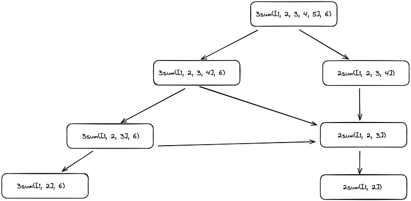
Overlapping Substructure: As I would realize if I tried to compute a length-5 array, this solution requires me to recompute 2Sum’s for the array each time I want to compute a 3Sum. Let’s write it similar to Fibonacci numbers.
3sum([1, 2, 3, 4, 5], 6) = 3sum([1, 2, 3, 4], 6) ++ 2sums([1, 2, 3, 4])
3sum([1, 2, 3, 4], 6) = 3sum([1, 2, 3], 6) ++ 2sums([1, 2, 3])

Whereas

2sums([1, 2, 3, 4]) = 2sums([1, 2, 3]) * 3
Instead of the actual functions, I have written the number of steps associated with each computation, but the realization should be that we are computing
2sums([1, 2, 3])
twice, one for computing
3sum([1, 2, 3, 4], 6)
and one for computing
2sums([1, 2, 3, 4])
, and in fact that’s a property of
2sums
. Any array that computes its 2sum always computes 2sums’s of all of its subsets.
Upon this realization, we will simply precompute 2sum and relieve ourselves of the responsibility of computing it every single time. Below is the actual code we would write for those who would like to test it by hand.
def two_sums(arr: list[int]) -> dict[int, tuple[int, int]]:
    """
    Returns a dictionary of all the two sums in the array
    """
    two_sum_dict = {}
    for i in range(len(arr)):
        for j in range(i + 1, len(arr)):
            if arr[i] + arr[j] not in two_sum_dict:
                two_sum_dict[arr[i] + arr[j]] = [(arr[i], arr[j])]
            else:
                two_sum_dict[arr[i] + arr[j]].append((arr[i], arr[j]))
    return two_sum_dict

def three_sum(arr: list[int], sum: int) -> list[int]:
    if len(arr) < 3:
        return []

    # Compute 3sum for the first part.
    c1 = three_sum(arr[:-1], sum)

    # Compute 2sum for the first part
    two_sum = two_sums(arr[:-1])

    # Check for all the pairs of numbers in the first part that conforms
    # to the given sum.
    c2 = list(map(lambda t: (t[0], t[1], arr[-1]), two_sum.get(sum - arr[-1], [])))

    # Merge two solutions
    return c1 + c2
The cached version is somewhat trickier and not as neat as the version I provide above.
def three_sum_cached(arr: list[int], sum: int, two_sums: dict[int, tuple[int, int]]) -> list[int]:
    if len(arr) < 3:
        return []

    # Same function call with the original version
    c1 = three_sum_cached(arr[:-1], sum, two_sums)

    # Instead of the function call, we lookup from the precomputed dictionary
    matching_two_sums = two_sums.get(sum - arr[-1], [])

    # This is to prevent using the same number twice
    filtered_two_sums = list(filter(lambda t: t[0] != arr[-1] and t[1] != arr[-1], matching_two_sums))

    c2 = list(map(lambda t: (t[0], t[1], arr[-1]), filtered_two_sums))
    # This is to prevent using the same triplets twice.
    # For example, we delete (1, 4, 3) and only leave (1, 3, 4)
    filtered_c2 = list(filter(lambda t: t[0] < t[1] < t[2], c2))

    return c1 + filtered_c2
The second algorithm is somewhat crude, but that’s probably on me. I bet there are better ways of implementing the caching.
Complexity: O(n²)(The time to compute the 2sums)
Visually, while the original looks similar to this:

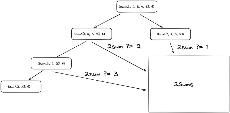
The cached implementation is similar to this:

2Sum part is kind of cheating as I’ve not written that part of the algorithm recursively, so it’s more similar to this:

Where 2Sums is the data structure that allows querying for tuples for a given amount in constant time.
Conclusion
In this article, I tried to convey my method/perspective on solving algorithmic problems using dynamic programming. My methodology rests on first creating a naive recursive solution for a problem with optimal substructures, identifying overlapping substructures and caching/memoizing those function calls. Hope it’s useful!